Execution Surplus and Welfare in a Simplified Intent-Auction Game
A better execution price tells us what a trader received, not what the market saved.
In an intent auction, solver competition and trader participation also determine which execution opportunities become available. This post asks how those forces, together with matching quality, shape private execution gains vs. aggregate welfare across batch durations.
The main piece is a Solver–Trader mechanism simulation under specified protocol fee, reward-cap, and batch-duration policies. Welfare accounting then separates transfers from real resource savings. A 25-order CoW audit in the Appendix marks which of those quantities public settlement data can identify; the simulation is not calibrated to those orders. Production CoW uses a fair combinatorial auction and a richer reward system (solving formulation; competition rules; rewards); the model uses a reduced-form winner reward capped as a share of fee revenue.
Actors, policy instruments, and payoffs
The model tracks three actor groups and five payoff categories. Protocol instruments are the fee , reward-cap share , and batch duration ; those policies are specified, while Solver effort and Trader participation are endogenous. Protocol profit is
where is participation, the Solver reward paid out, and operating cost. Two Solvers choose efforts on a discrete grid; the higher-effort Solver wins , and equal efforts pay zero to both:
where is the effort-cost parameter. Joint Solver profit is . A unit mass of traders chooses immediate AMM execution or the intent venue:
where is private friction avoided by a successful match, matching quality, and the last term expected waiting cost under unit-time costs uniform on with expected delay . The all-pay cost structure follows complete-information contests such as Baye, Kovenock, and de Vries (1996); quadratic cost and a deterministic winner are modeling choices.
| Actor | Role in the reported exercises |
|---|---|
| Protocol | Sets ; profit evaluated under that policy |
| Solvers | Choose on the effort grid; payoffs |
| Traders | Choose AMM now vs. intent batch; aggregate payoff |
| LP / MEV | Passive incidence (foregone outside-route revenue), not strategic |
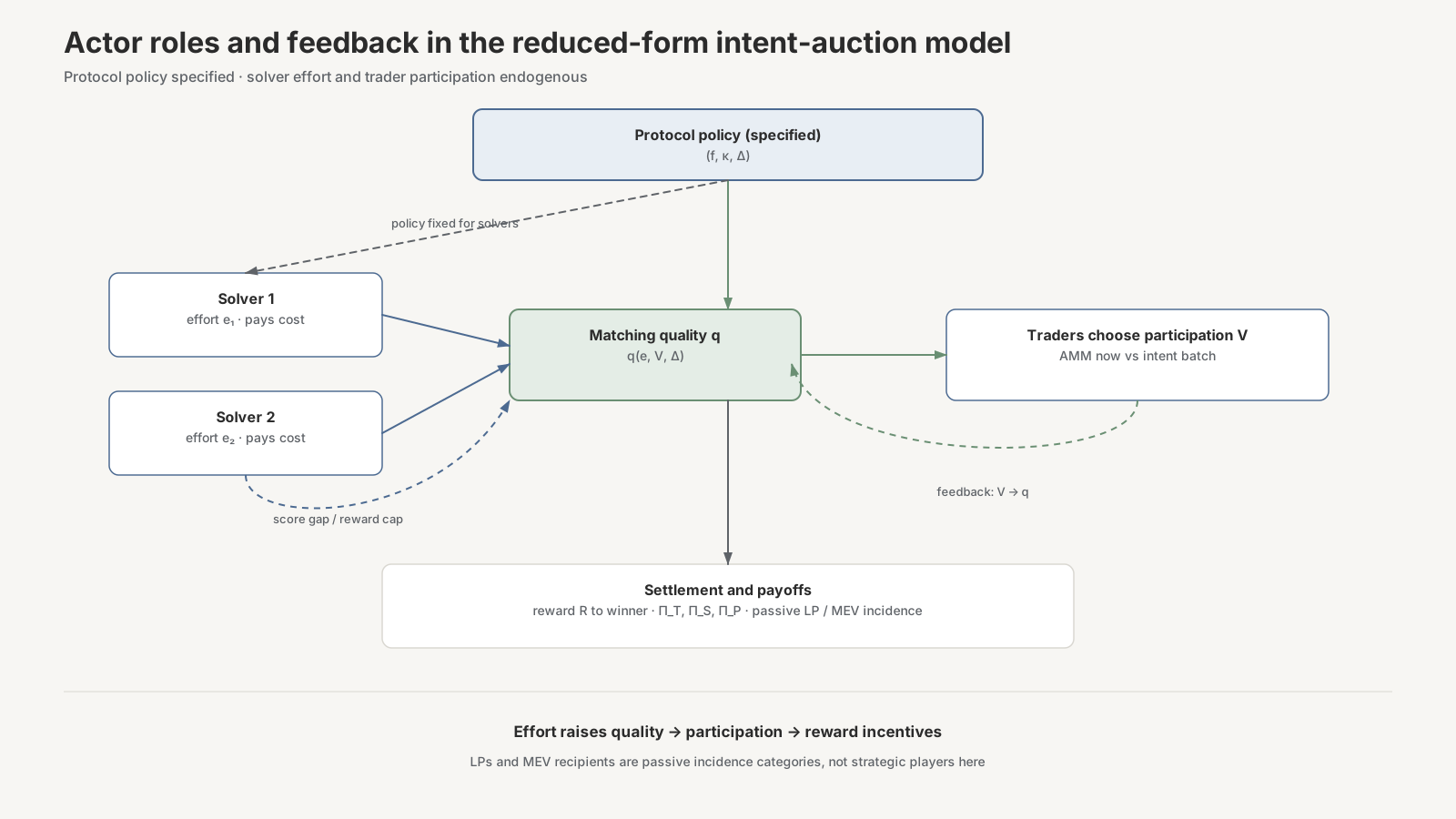
Fig. 1. Actor roles and feedback: Solver effort raises matching quality, which shifts participation and feeds back into Solver rewards. Batching complementarities: Canidio and Henneke.
Matching, participation, and equilibrium selection
Matching quality is
where is baseline match probability, a baseline matching intensity, and the effort sensitivity of that intensity. Given an effort profile, set . Participation is the highest locally stable fixed point of
Denote that root by . Both Solvers are then scored at the same :
If , the winner reward is
where converts the quality gap into a reward; if , both rewards are zero. A unilateral deviation recomputes , re-solves under the same highest-stable-root rule, and reassigns rewards. Thickness–waiting trade-offs in dynamic matching markets motivate treating delay as economically meaningful (Akbarpour, Li, and Oveis Gharan, 2020); the functional form is a modeling assumption.
For fixed , the simulation enumerates efforts on . A pure-grid Nash equilibrium has no profitable unilateral deviation on that grid. If several equilibria exist, selection maximizes joint Solver payoff , then matching quality , then lexicographically minimizes . Sampled durations without a pure-grid equilibrium are marked unavailable. Duration scans fix and and vary only . Baseline primitives (, , ) and market compositions are reported in the companion notebook. With and , is a meaningful baseline participation boundary in this specification: if matching quality cannot clear that hurdle, the selected outcome can be .
Batch duration in the Solver–Trader subgame
A longer batch allows more time for matching but raises waiting costs; participation responds to both. Frequent batch auctions motivate treating the interval as a design object. Here stay fixed while Solvers and Traders adjust: Protocol profit tracks fees net of rewards, while aggregate welfare tracks avoided real resource cost net of waiting, Solver effort, and operating cost. Figures below compare two markets that keep the same private friction but split it differently into transfers vs. real resources (transfer-heavy vs. resource-heavy; compositions in the companion notebook).
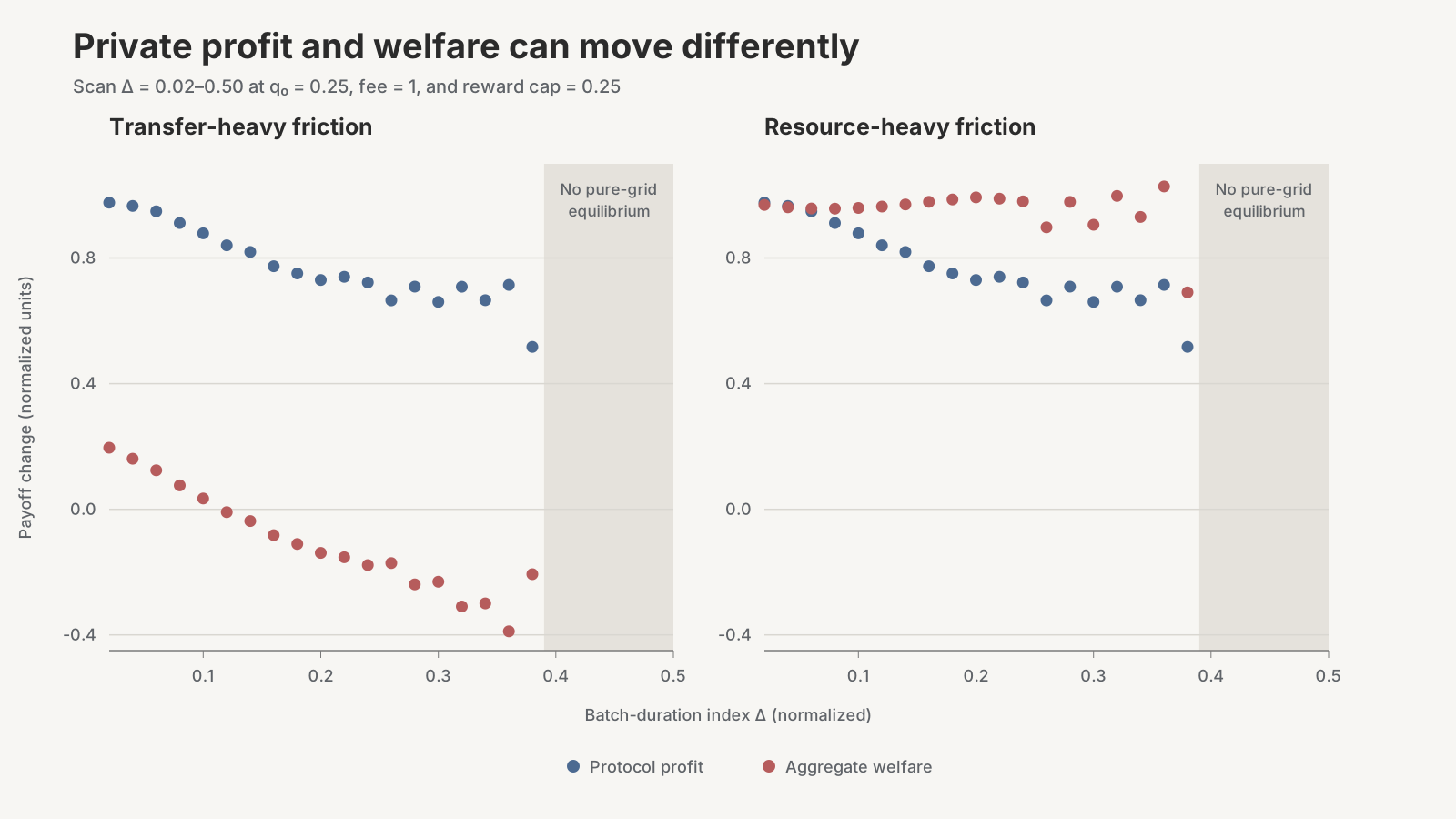
Fig. 2. Selected pure-grid equilibria over Δ=0.02–0.50 with f=1 and κ=0.25. Points are unconnected (discrete effort and participation). Shaded durations have no pure-grid equilibrium. At Δ=0.38, selected V=0.716.
Between and , the selected equilibrium moves from effort and full participation to effort and participation of approximately . Matching quality rises from to . In the resource-heavy specification, the resulting increase in avoided real costs exceeds the additional waiting and effort costs. Welfare increases modestly from to , while Protocol profit falls from to . Endogenous participation also changes equilibrium availability in the discrete solver contest (19 vs. 12 of 25 sampled durations). This result is sensitive to the contest specification and is not a general equilibrium-existence claim; the full endogenous vs. fixed comparison is in the companion notebook.
Varying only shows a related participation boundary. Lower can raise the relative importance of batch duration when positive-participation equilibria remain; it can also produce selected pure-grid equilibria with .
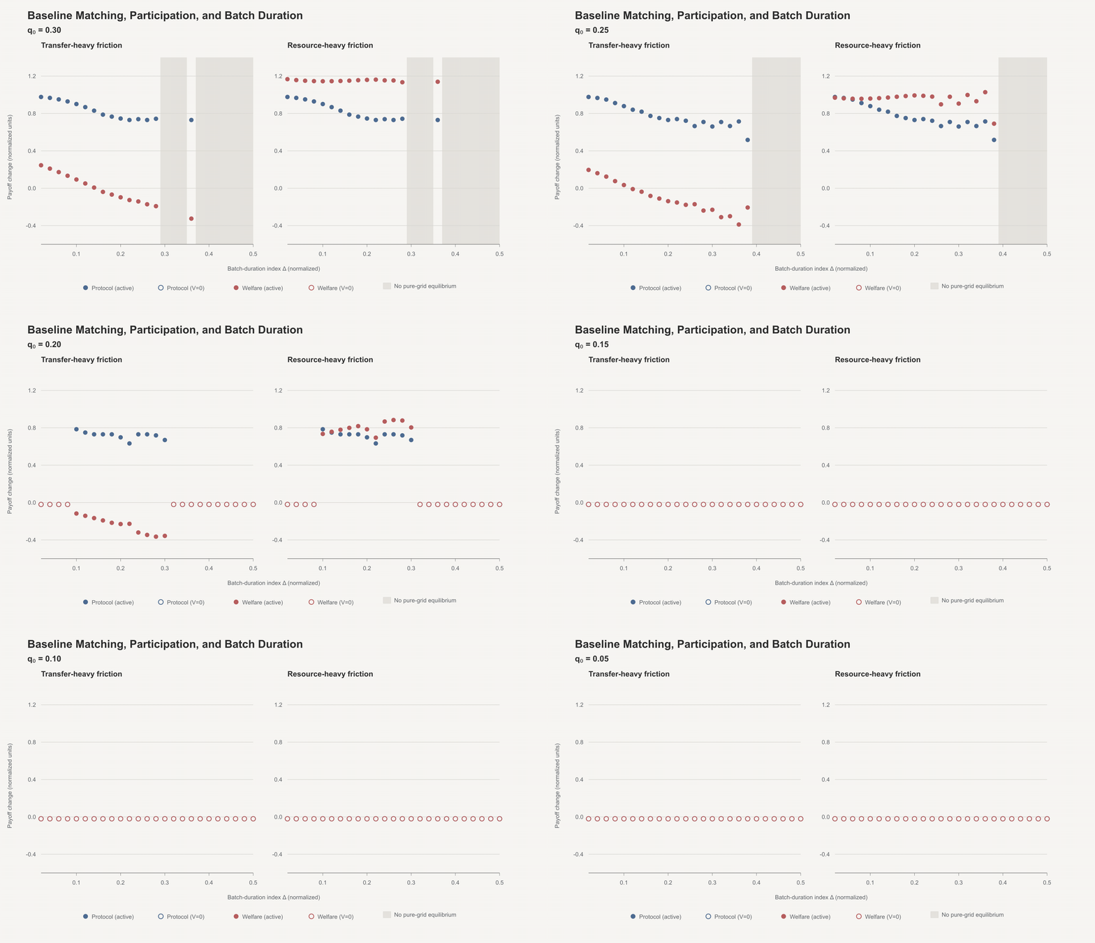
Fig. 3. Only q₀ changes (0.30→0.05); f=1, κ=0.25, Δ grid, and selection fixed. Filled = V>0 equilibrium; hollow = selected V=0; gray = no pure-grid equilibrium. On this grid, resource-heavy welfare peaks at Δ=0.02 when q₀=0.30 and at Δ=0.36 when q₀=0.25; for q₀≤0.15 every selected outcome has V=0.
Welfare accounting: transfers vs. resources
with avoided LP fee revenue, avoided trader-borne extraction, and avoided real resource cost. After transfers cancel,
Private payoffs depend on , not its split, so changing the composition leaves the selected equilibrium unchanged and
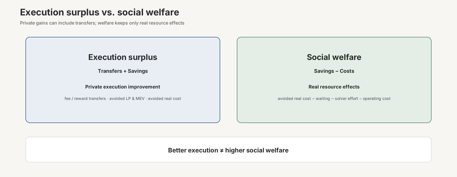
Fig. 4. Private execution improvement can include transfers; keeps only real-resource savings net of waiting, Solver effort, and operating cost. Ledger detail: companion notebook.
At , , the selected allocation is , , efforts , , . Holding that allocation fixed and changing only the composition of :
| Actor | Transfer-heavy | Resource-heavy |
|---|---|---|
| Trader | +0.486 | +0.486 |
| Solver | +0.154 | +0.154 |
| Protocol | +0.730 | +0.730 |
| LP | −0.755 | −0.189 |
| MEV recipient | −0.755 | −0.189 |
| Social welfare | −0.139 | +0.993 |
Private payoffs are identical; reverses sign with the resource share. Whether public CoW data can identify that split is a separate question; the Appendix records a 25-order identification audit and one shared-settlement worked example.
Closing
Better execution is a private outcome, not a welfare measure. The open measurement problem is the resource share of execution surplus: without it, a private edge cannot be mapped to . The audit below is a scope check on that gap, not a calibration of the game.
Appendix
Baseline parameters, market compositions, and reproduction checks are in the companion notebook.
On-chain data audit: 25 CoW orders
Separately from the simulation, I examined 25 executed Ethereum orders across 23 CoW settlements. Each order has a direct Uniswap v3 quote at the exact auction-start block; 23 records expose protocol-fee arrays. Twenty quotes selected a 1 bp pool and five a 5 bps pool. These are benchmark route choices, not confirmed bilateral CoW matches.
Worked example (shared settlement)
Settlement 0x17868a…d60def contains two audited orders at auction-start block 25715500. Focus on order 0x06782a…81ef0 (USDC→WETH sell):
| Observed field | What it establishes | What remains unidentified |
|---|---|---|
Order UID 0x06782a…81ef0 | Unique executed order | Trader valuation / waiting cost |
Settlement tx 0x17868a…d60def | Shared settlement with a second order | Bilateral vs. buffer vs. external liquidity |
Auction-start block 25715500 | Quote timing state | Full outside-route opportunity set |
Uniswap v3 quote (1 bp): 0.008568443238783844 WETH (8,568,443,238,783,844 wei). Reconstructed by eth_call against the pool quoter at block 25715500—there is no separate quote transaction | Narrow same-block direct-pool benchmark | Whether that pool was the relevant outside option |
CoW executed buy: 0.008591511028597428 WETH (8,591,511,028,597,428 wei), recorded on order 0x06782a…81ef0 and settlement 0x17868a…d60def | Private execution vs. that quote (+26.9 bps archived edge) | Transfer vs. resource split of the edge |
| Protocol-fee policy array (present) | Fee-policy fields were exposed | Recipient reconciliation and incidence |
Settlement gas used 193,784; effectiveGasPrice 156,112,596 wei (≈0.156 gwei); payment 30,252,123,303,264 wei (= gasUsed × effectiveGasPrice) from eth_getTransactionReceipt | Settlement-level gas expenditure in wei (field is not gwei) | Order-level allocation; transfer vs. real-resource share of gas |
The receipt reports settlement-level gas, not an order allocation. Charging the full payment to each of two co-settled orders would imply
where is the settlement gas payment. Sharing a settlement does not identify bilateral matching; matching_class is unavailable here, so the edge cannot be split into and .
Across the probe, realized solver rewards, losing-solvers' resource costs, and traders' waiting disutility are unobserved. Public data support a narrow execution-quality comparison and a limited fee/gas availability check—not the empirical resource share of surplus.
Notes
- Code. Companion notebook (baseline parameters, welfare ledger, incidence, duration scans, endogenous-vs-fixed table); fixed-participation scan:
scripts/compare_fixed_participation.py. - Audit source.
results/cow_welfare_identification_pilot/opportunity_probe_25.csv. - CoW sources. Solving formulation; competition rules; rewards.
- Primary references. Canidio and Henneke; Akbarpour, Li, and Oveis Gharan (2020); Budish, Cramton, and Shim (2015); Baye, Kovenock, and de Vries (1996).
- Related. Loss-Versus-Rebalancing, RediSwap, and Ota's order-by-order auction model.