TVL, Marginal Price, and Liquidity in an AMM

TVL is a measure of capital. The marginal price is the current quote. Liquidity tells us how much trading it takes to move that quote.

A pool page can show a large total value locked (TVL) and an attractive Ether (ETH) price, yet neither number tells me what will happen if I actually send a large order.

Automated market makers (AMMs) are often discussed from the liquidity-provider (LP) side—fees, inventory, and position value. I will look at the same pool from the trader’s side: not only what capital sits there or what price appears on screen, but what happens when I actually trade against it.

Most drawings are constructed. A later section checks the distinction against a real Uniswap v3 pool at a fixed block.

TVL: how much capital sits behind the pool?

Take a pool holding 100 ETH and 200,000 USD Coin (USDC). If ETH is marked at \$2,000 and USDC at one dollar, the inventory is worth about \$400,000.

That number can rise because more tokens enter the pool. It can also rise with no deposit at all: if an external USD mark for ETH rises to \$2,500 while the pool inventory itself is unchanged, the marked value becomes \$450,000.

TVL tells me something about the amount of marked capital associated with the market, but not yet what my order will receive.

Marginal price: what quote do I face for a tiny trade?

An AMM does not store a price tag. It stores a rule for how its reserves can change. For a constant-product pool, ignoring fees,

\[ xy = k. \]

A trade changes $x$ and $y$, but keeps the pool on that curve. The reserve ratio gives the marginal quote:

\[ p = \frac{y}{x}. \]

So 100 ETH against 200,000 USDC and 40 ETH against 80,000 USDC can both quote \$2,000. The reserves are very different; the ratio is the same.

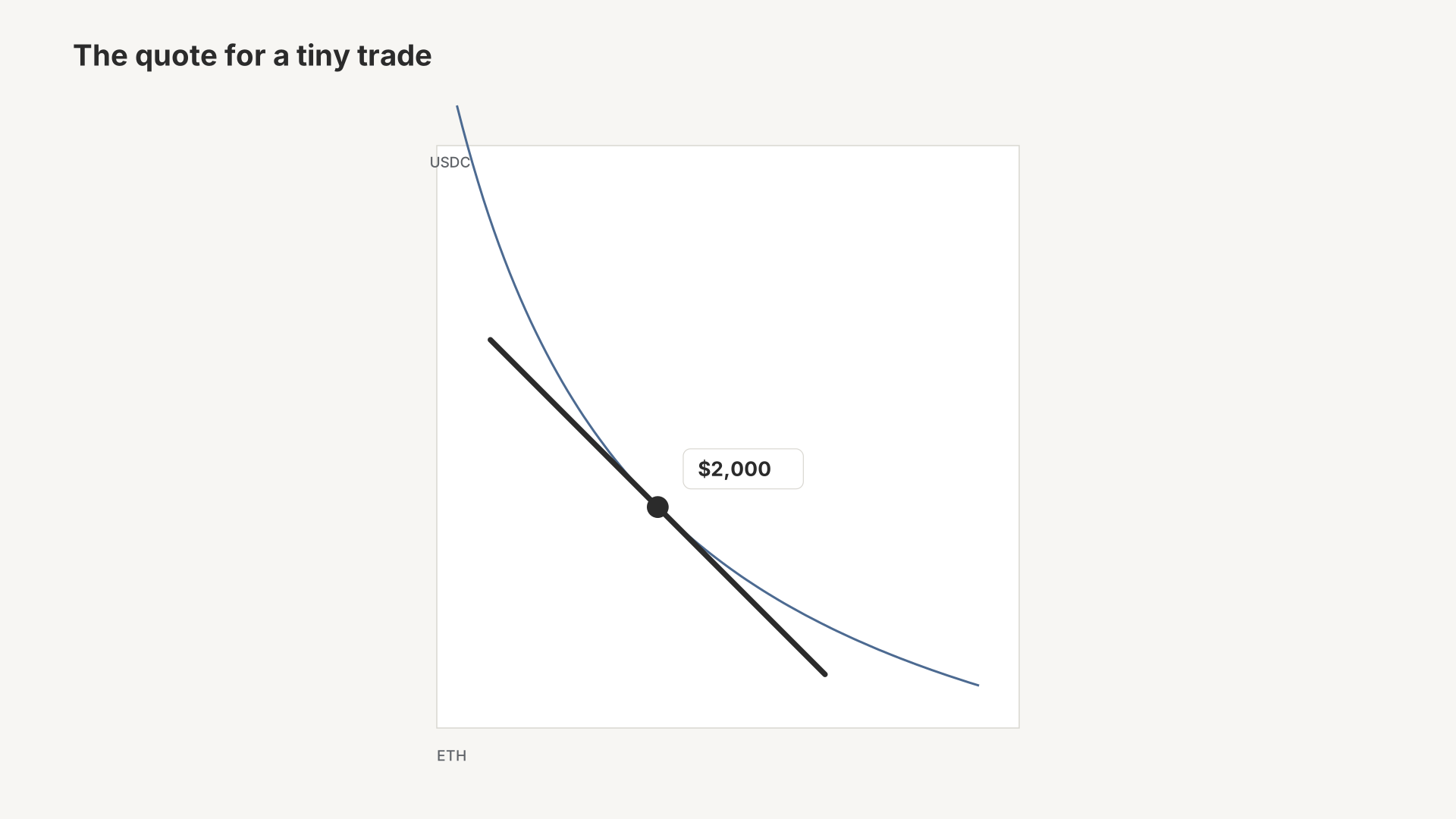
The curve in Fig. 1 is the constraint. The dot is the current state. The tangent is a geometric way to see the quote at that state.

Fig. 1. Fee-less constant-product example. The absolute slope of the tangent is the marginal quote: 2,000 USDC per ETH.

A live pool charges a fee, so the next buy and sell sit a little off this ratio. The pictures leave fees out. The general form of the rule for pools that are not constant-product is in the appendix.

I used the same idea in an earlier pool-state experiment: once the reserve state is reconstructed, the quote and the effect of the next trade follow from that state. That note is Before MEV, I Built a Rust AMM Lab to Measure Pool State.

Liquidity: what changes when my order is no longer small?

The marginal price is a local number. It describes the next small piece of the trade. Liquidity tells me how much size is needed to move the quote by a given amount.

Suppose two pools both start at \$2,000 per ETH. One holds 10 ETH and 20,000 USDC; the other holds one hundred times as much. Send the same \$10,000 buy to both. In the small pool, the marginal quote ends at \$4,500. In the large pool, it barely reaches \$2,020.

The starting price was the same. What differed was how much size each market could take before the quote moved beyond a given level. The exact steps are in the appendix.

That is the trader-facing quantity: how much of the order can execute before a chosen amount of price impact. The answer depends on the reserve state and, in concentrated pools, on which positions are active at the current price.

Now put the three together

The same buy, a bigger pool

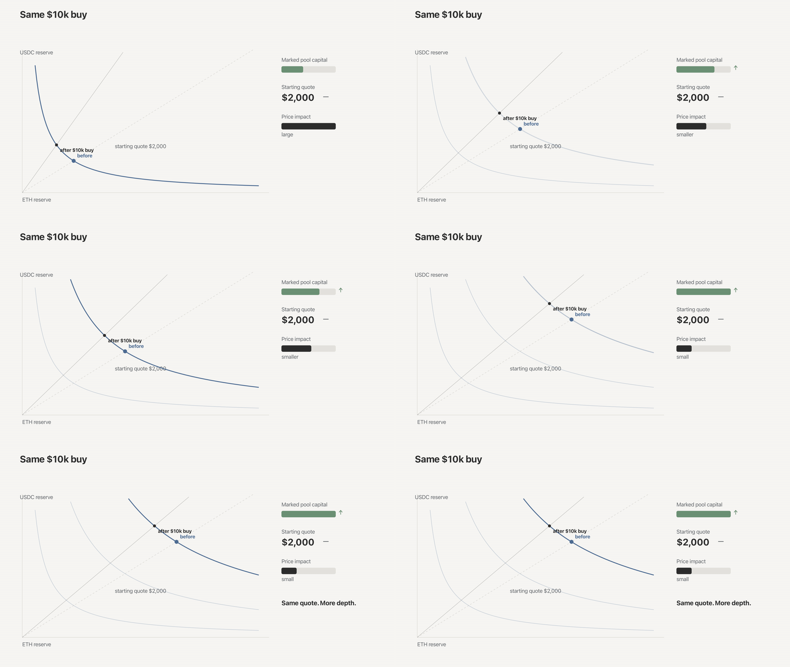
Start with the easiest case. Scale the reserves without changing their ratio. Fig. 2 applies the same \$10,000 buy. Marked pool capital rises, the starting quote remains \$2,000, and the order moves it less: from \$4,500 on the small pool to about \$2,722 once reserves are three times as large.

Animation of the same 10,000 dollar buy against a growing pool. A capital bar fills, the starting quote stays at 2,000 dollars, and a price-impact bar shrinks.

Fig. 2. Fee-less constant-product example. At a \$2,000 ETH mark, marked pool capital rises from \$40,000 to \$120,000.

I send the order

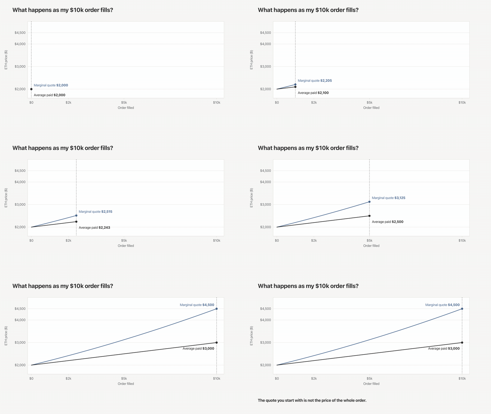
Now hold the pool fixed and change the order instead. A \$2,000 marginal quote does not mean a \$10,000 order will execute at \$2,000. Fig. 3 follows the order as it fills. The quote for the next small piece rises faster than the average price already paid.

By the end of this constructed trade, the pool is quoting \$4,500 while the order itself averaged \$3,000. The number on screen is the starting point of execution, not a promise for the whole order.

Animation of two lines against dollars filled, from 0 to 10,000. The marginal quote rises from 2,000 to 4,500 dollars. Average paid rises from 2,000 to 3,000. Labels sit on the line ends.

Fig. 3. Fee-less constant-product example. The x-axis is cumulative order size, not time.

Here the state change sits on one curve. In an earlier Uniswap quote ladder, larger orders began to use more pools and intermediate hops. The routing changed because usable depth depends on size. That measurement is in The Price Moves First. DEX Routes Fray Before the Exit.

Depth can change during the order

Concentrated liquidity adds one more possibility: the depth available to the next dollar of my trade can itself change as the quote moves. A pool can contain a great deal of capital that my trade cannot use at the current price.

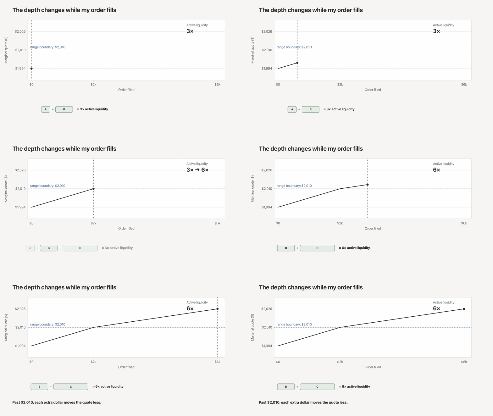
Active liquidity tells me how much size is needed to move the current quote. In Fig. 4, positions A and B are active around \$1,994, providing 3× of schematic active liquidity. At the \$2,010 range boundary, A ends and the larger position C begins. Active liquidity becomes 6×.

The quote does not jump at the boundary. What changes is how quickly the next dollars of the order move it.

Animation of a marginal quote against dollars filled. The path is steeper until 2,010 dollars, then flattens as active liquidity goes from 3× to 6×.

Fig. 4. Relative liquidity levels are schematic; the fee-less price path follows concentrated-liquidity swap mechanics.

TVL values the capital across the pool. Active liquidity tells me what matters here, at this price, for the next part of my trade.

One pool, one block

The examples above are constructed. The distinction also shows up in a real pool.

At Ethereum block 26,138,774, the Uniswap v3 USDC/wrapped Ether (WETH) 0.05% pool 0x88e6…5640 held about 72.4 million USDC and 9,453 WETH. Dividing those balances gives roughly \$7,663 per WETH. The pool’s marginal quote at that block was about \$2,620.

The gap reflects how v3 represents price and liquidity; it is not an inconsistency in the pool. Aggregate token balances are not the reserve pair used to recover the current quote. If I mark the contract-held balances at the pool’s own marginal price, their value is about \$97.2 million. That is a mark-to-market valuation of the contract-held inventory, not a measure of the depth available to my next order.

Closing

TVL is a starting point. A large pool can still be thin at the price I care about, and a good marginal quote can deteriorate quickly once the order has size.

For a trader, the useful question is not simply how much capital the pool contains. It is how much size I can execute, in this direction, before price impact exceeds what I am willing to pay.

That is the quantity I later measured as executable capacity across sibling Uniswap v3 pools in When Multiple Pools Behave Like One: Impact-Constrained Capacity Concentration in Uniswap v3.

Appendix

All constructed examples ignore fees. The constant-product examples use $xy=k$: the same \$10,000 buy ends at a \$4,500 marginal quote in the small pool and near \$2,020 in the pool 100× larger. Scaling reserves 1×→3× preserves the \$2,000 quote while marked pool capital rises from \$40,000 to \$120,000.

Fig. 4 is schematic. At \$2,010, active liquidity changes from 3× to 6×; under its chosen price orientation, quote-token input is $L(\sqrt{Q}-\sqrt{P})$. This normalization is separate from the real pool’s token0/token1 ordering.

The real-pool reading uses the Uniswap v3 USDC/WETH 0.05% pool, 0x88e6…5640, at Ethereum block 26,138,774. TVL conventions vary across interfaces. How Uniswap works · Concentrated liquidity.